Markov Decision Process
# Components of MDP
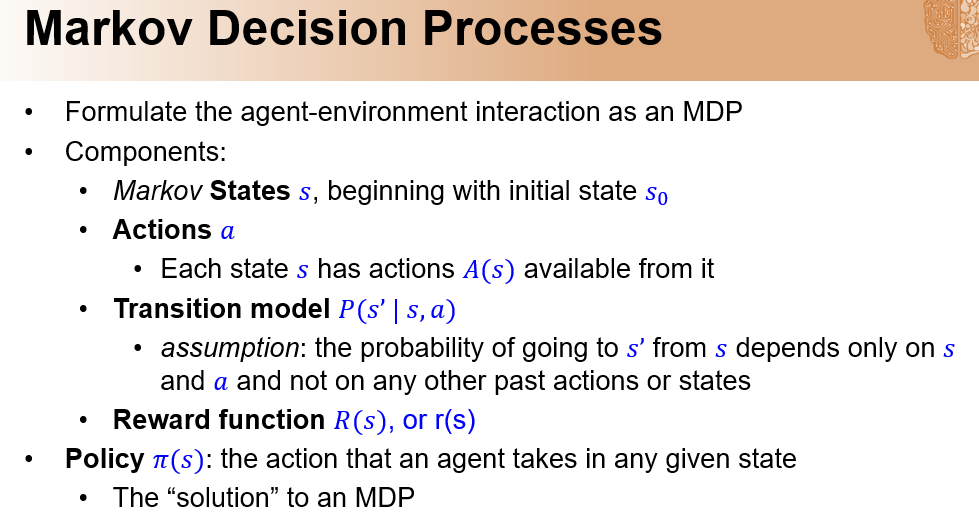
# Formulating an MDP


# The Bellman Equation
$$ V_{i+s}(s) =max_a(\sum_{s’} P(s’|s,a)(r(s,a,s’)+\gamma V(s’)) $$
# Value iteration
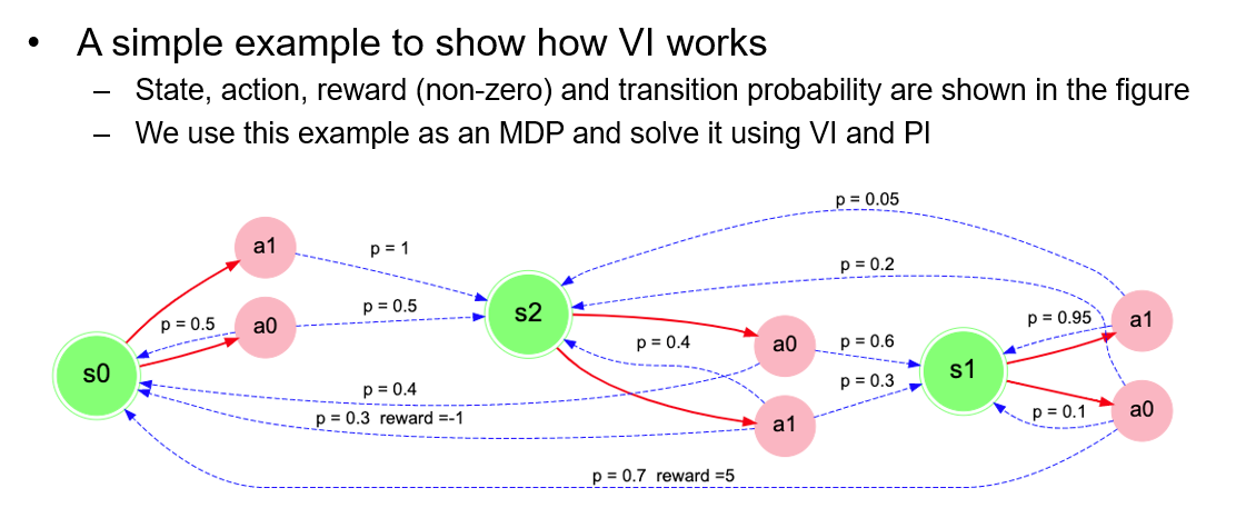
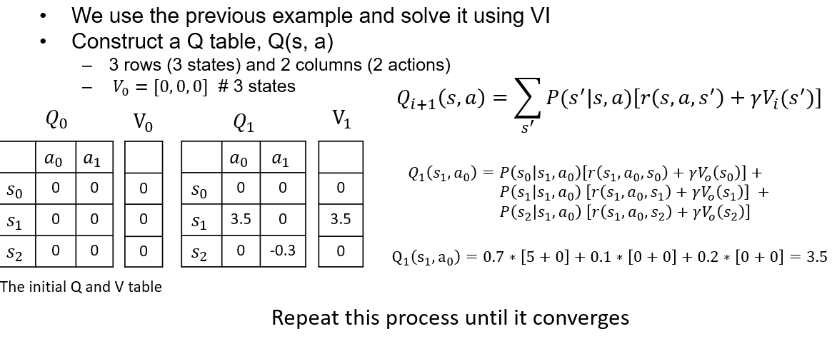
| $V_i$ | (1,1) | (1,2) | (1,3) | (2,1) | (2,2) | (2,3) |
|---|---|---|---|---|---|---|
| $V_0$ | 0 | 0 | 0 | 0 | 0 | 0 |
| $V_1$ | 0 | 0 | 0 | 0 | $Up = 0.8\times0+0.1\times5+0.1\times0+0.9\times0$ $Down=0.8\times0+0.1\times5+0.1\times0+0.9\times0$ $Left=0.80+0.15+0.10=0.5$ $Right=0.85+0.10+0.10=4$ Max = 4 | 0 |
| $V_2$ | 0 | $Up=0.8\times(0+0.9*4)+$ $0.1\times0+0.1\times-5=2.38$ | 0 | $Right=0.8\times(0+0.9*4)+$ $0.1\times0+0.1\times0=2.88$ | $Right=0.8\times(5+0.90)+$ $0.1\times(0+0.94)=4.36$ | 0 |
# Obtain the optimal policy
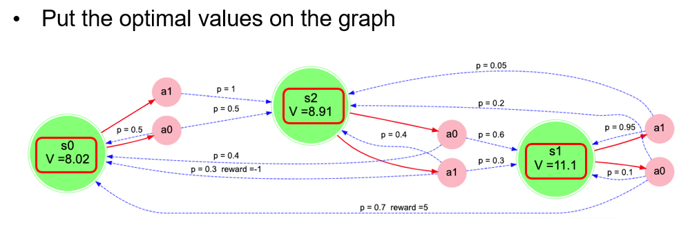
Once we have V*, we can use V* in the bellman equation for each State and Action to obtain the corresponding Q(S,A) value. $\pi*$ is the action which obtains max Q(S,A) i.e. V(S).

# Policy iteration
Steps
- Start with random policy and V(s)=0 for 1st iteration
- Policy evaluation (calculate V) until stable 1. For each state s calculate V(s) using the action in the policy (this is different from calculating V(s) using max $Q(s,a)$)
- Policy Improvement (calculate new policy) 1. For each state s calculate $Q(s,a)$ of all actions using the stabilized V(s) values. 2. Update the policy with the actions which maximize $Q(s,a)$ of each state
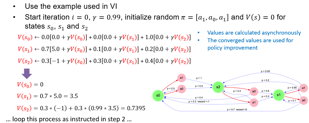 Asynchronous refers to in series: value calculated from previous steps (same iteration) are used in the next state calculations.
Synchronous refers to in parallel: All V(s) values are calculated using the previous iteration V(s) estimates.
Without the transition function or probabilities we need Monte Carlo Policy reinforcement learning.